
Modern Portfolio Theory, Monte Carlo Simulations & CVaR for Smarter Investment Decisions
Maximize Returns and Minimize Risks Using Advanced Financial Modeling Techniques


Introduction
Investing is both an art and a science. It’s about finding that perfect balance between risk and return. Modern portfolio theory offers powerful tools to help investors achieve this balance, utilizing optimization techniques to select an ideal mix of assets. In this post, we’ll walk through a complete implementation of portfolio optimization and Monte Carlo simulations, explaining each step and illustrating the results with insightful visualizations.
We’ll cover everything from calculating expected returns and optimizing portfolios for the maximum Sharpe ratio to analyzing risk using Monte Carlo simulations and assessing Value at Risk (VaR). Let’s dive in!
Step 1: Import Data from Yahoo Finance
We start by collecting historical stock price data for five popular companies: Apple (AAPL), Microsoft (MSFT), Alphabet (GOOGL), Amazon (AMZN), and Tesla (TSLA). Using Yahoo Finance, we gather the adjusted closing prices between January 1, 2018, and January 1, 2023.
# List of stock tickers
tickers = ['AAPL', 'MSFT', 'GOOGL', 'AMZN', 'TSLA']

# Define the start and end date
start_date = '2018-01-01'
end_date = '2023-01-01'

# Download the adjusted closing prices
data = yf.download(tickers, start=start_date, end=end_date)['Adj Close']
Step 2: Calculate Daily Returns
To understand each stock’s behavior over time, we calculate the daily returns:
# Calculate daily returns
returns = data.pct_change().dropna()
Step 3: Calculate Expected Returns and Covariance Matrix
Next, we calculate the expected annual returns and covariance matrix, which are essential inputs for portfolio optimization.
# Calculate expected returns and covariance matrix (annualized)
expected_returns = returns.mean() * 252
cov_matrix = returns.cov() * 252
Step 4: Portfolio Optimization for Maximum Sharpe Ratio
Our goal is to build an optimal portfolio. The Sharpe ratio is a key metric, representing the ratio of return to risk (volatility). We use optimization techniques to find the portfolio allocation that maximizes the Sharpe ratio.
def portfolio_annualised_performance(weights, mean_returns, cov_matrix):
    returns = np.sum(mean_returns * weights )
    std = np.sqrt(np.dot(weights.T, np.dot(cov_matrix, weights)))
    return std, returns

def negative_sharpe_ratio(weights, mean_returns, cov_matrix, risk_free_rate):
    p_var, p_ret = portfolio_annualised_performance(weights, mean_returns, cov_matrix)
    return -(p_ret - risk_free_rate) / p_var

def max_sharpe_ratio(mean_returns, cov_matrix, risk_free_rate):
    num_assets = len(mean_returns)
    args = (mean_returns, cov_matrix, risk_free_rate)
    constraints = ({'type': 'eq', 'fun': lambda x: np.sum(x) - 1}) # Sum of weights is 1
    bounds = tuple((0,1) for asset in range(num_assets)) # No short selling
    result = minimize(negative_sharpe_ratio, num_assets*[1./num_assets,], args=args,
                      method='SLSQP', bounds=bounds, constraints=constraints)
    return result

def portfolio_volatility(weights, mean_returns, cov_matrix):
    return portfolio_annualised_performance(weights, mean_returns, cov_matrix)[0]

def efficient_return(mean_returns, cov_matrix, target):
    num_assets = len(mean_returns)
    args = (mean_returns, cov_matrix)

    def portfolio_return(weights):
        return np.sum(mean_returns * weights)

    constraints = ({'type':'eq', 'fun': lambda x: portfolio_return(x) - target},
                   {'type':'eq', 'fun': lambda x: np.sum(x) - 1})
    bounds = tuple((0,1) for asset in range(num_assets))
    result = minimize(portfolio_volatility, num_assets*[1./num_assets,], args=args,
                      method='SLSQP', bounds=bounds, constraints=constraints)
    return result

def efficient_frontier(mean_returns, cov_matrix, returns_range):
    efficients = []
    for ret in returns_range:
        efficients.append(efficient_return(mean_returns, cov_matrix, ret))
    return efficients
Maximum Sharpe Ratio Portfolio Allocation Annualised Return: 36.14 % Annualised Volatility: 35.18 % Allocation: allocation Ticker AAPL 34.31 AMZN 0.00 GOOGL 0.00 MSFT 36.23 TSLA 29.46
Step 5: Plotting the Efficient Frontier
To understand the trade-off between risk and return, we plot the Efficient Frontier, which shows the optimal portfolios for various levels of expected return.
The graph below illustrates:
The efficient frontier (in black).
Individual assets plotted as 'X' marks.
The maximum Sharpe ratio portfolio represented by a red star.
We also generate random portfolios for context, providing a view of the distribution of potential portfolios.
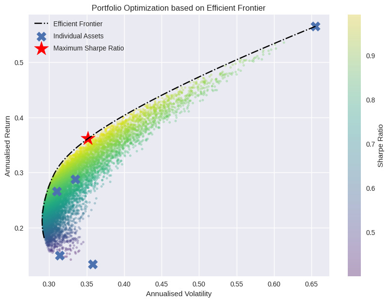
This plot helps visualize the portfolio combinations that maximize return for each level of risk, allowing investors to make informed choices.
Step 6: Monte Carlo Simulation for Scenario Analysis
After constructing the optimal portfolio, we perform Monte Carlo simulations to explore different future scenarios for portfolio value. We simulate 1,000 different paths for the portfolio value over a 1-year time horizon.
# Monte Carlo Simulation
portfolio_simulations = monte_carlo_portfolio_simulation(start_price=1000000, daily_mean_returns.values, daily_cov_matrix.values, max_sharpe['x'], num_simulations=1000, time_horizon=252)
The results, plotted below, illustrate how the value of a $1,000,000 portfolio could evolve under various market conditions.
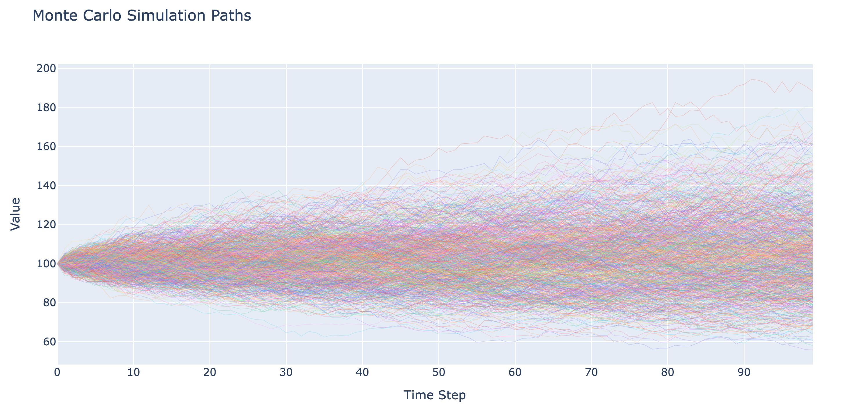
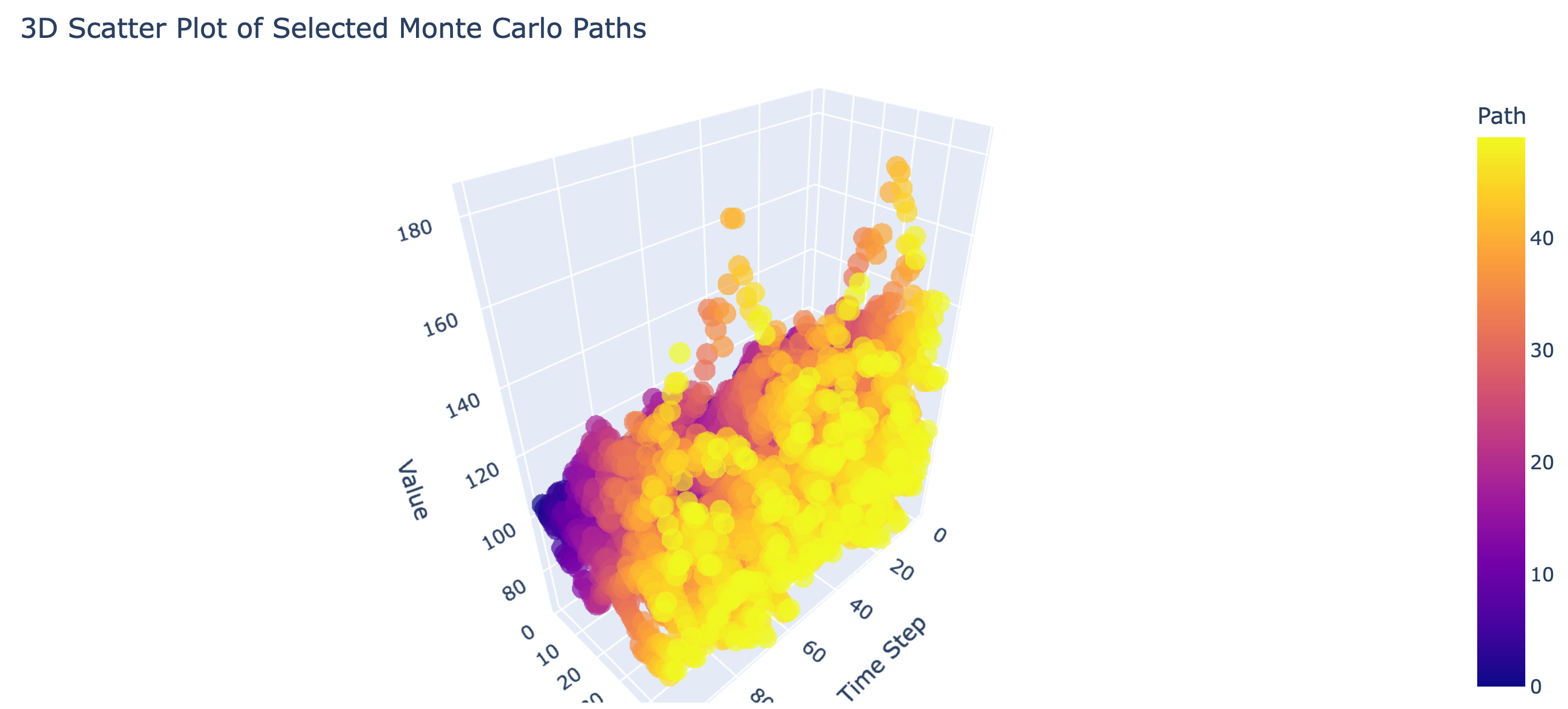
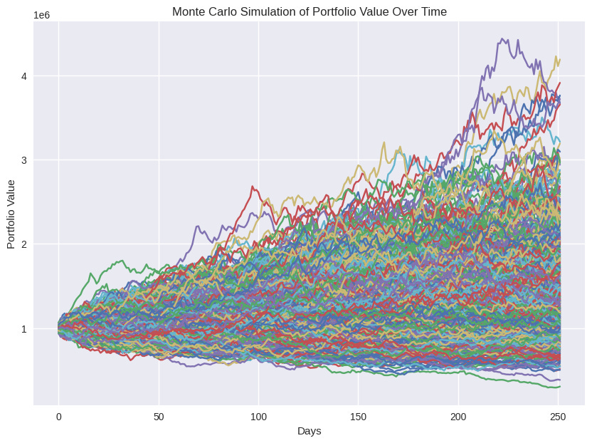
Monte Carlo simulations help investors understand potential outcomes and the variability of portfolio performance, providing a realistic view of risks.
Step 7: Risk Analysis with VaR and CVaR
To evaluate the downside risk, we calculate the Value at Risk (VaR) and Conditional Value at Risk (CVaR) at a 95% confidence level. These metrics help quantify the potential losses and the average loss beyond the VaR threshold.
# Value at Risk (95% confidence)
percentile_95 = np.percentile(ending_values, 5)
VaR_95 = start_price - percentile_95

# Conditional Value at Risk (95% confidence)
cvar_95 = start_price - ending_values[ending_values <= percentile_95].mean()

print(f"Value at Risk (95% confidence): ${VaR_95:,.2f}")
print(f"Conditional Value at Risk (95% confidence): ${cvar_95:,.2f}")
Results:
Value at Risk (95% confidence): $262,452.28
Conditional Value at Risk (95% confidence): $349,361.21
These risk metrics provide a critical view of the portfolio’s downside risk, helping investors prepare for worst-case scenarios.
Conclusion
Through the combination of portfolio optimization and Monte Carlo simulations, we can gain a deeper understanding of risk and return dynamics. The optimization techniques help us create an efficient portfolio, while scenario analysis and risk metrics like VaR and CVaR offer valuable insights into potential future outcomes.
Whether you’re an experienced investor or a beginner, understanding these tools will help you make more informed decisions, achieve better diversification, and align your investments with your risk tolerance.
Key Takeaways:
Efficient Frontier: Balances risk and return, guiding asset allocation decisions.
Monte Carlo Simulations: Assess the variability of portfolio performance over time.
Risk Metrics (VaR and CVaR): Provide insight into potential losses under adverse conditions.
We hope this post has helped demystify some of the complexities of portfolio optimization and risk analysis. Feel free to try this code yourself, adjust the parameters, and explore how different factors affect portfolio performance.